
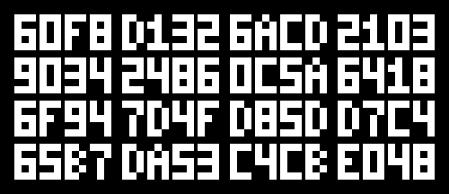
Remember the FORCEDENTRY exploit? Its strangest trick paired a memory-corruption bug with more than 70,000 JBIG2 bitmap operations to build a tiny computer inside an image decoder. The same general idea — building weird machines from behavior already present in a parser or decoder — can surface across file formats, protocol handlers, and plenty of other attack surfaces. It mostly remains the domain of the highest-level cool kids in exploit development: people who can look at a file format and see an instruction set hiding inside it.
This project takes that idea into JPEG XL through documented format behavior. The Meta-Adaptive tree supplies branches, optional channels carry state, raster coordinates set the execution order, and decoded 31-bit samples act as machine words. Package all of that into an ordinary JXL codestream, hand it to a stock decoder, and the decoder runs the program while reconstructing the image above.
Let’s start with the punchline. Hash the complete file and you get:
60f8d1326acd2103903424860c5a64186f947d4fd85dd7c465b7da53c4cbe048
Decode those exact same bytes and the pixels display:
60F8D1326ACD2103
903424860C5A6418
6F947D4FD85DD7C4
65B7DA53C4CBE048
Same value, just uppercase. The decoder computes those digest bits, passes them through a font ROM encoded in the JXL, and draws every glyph.
Get the artifact
The exact 11,714,152-byte file described in this post. Hash it, decode it with stock djxl, and check the pixels yourself.
The CPU executes one purpose-built program. It starts from a SHA-256 chaining state embedded by the authoring tool, runs the final compression block, routes the resulting 32 bytes into hexadecimal nibbles, and drives a pixel font. The result is a hashquine: a file whose decoded content represents a hash of the complete file, including the data that makes the representation appear.
Start with a read-once branching program
Start with a Boolean function and imagine computing it by asking questions such as “is input bit 7 zero or one?” Each internal node contains a question and has two outgoing edges. Evaluation follows the chosen edge until it reaches a terminal node containing the result.
A branching program generalizes the tree into a directed acyclic graph. Different decision paths may converge on the same later node, so common work can be shared. Its width measures how many distinguishable states it can hold at one layer; its length or depth measures how many rounds of questions it performs.
A read-once branching program, or ROBP, imposes a useful restriction: along a path from the entry to a terminal, each logical input variable is examined at most once. In the common ordered form, every path encounters variables in the same order. Their natural strength is streaming computation: read a symbol, update finite state, and continue forward.
An ROBP behaves like a pre-wired circuit. The questions arrive in a known order, each answer selects the next path, and the path taken carries the machine’s state. That is almost exactly the shape we need inside a raster decoder.

JPEG XL gives this abstract model a physical layout. Samples are reconstructed in a fixed order. The Meta-Adaptive tree chooses an operation from coordinates, channel identity, and previously reconstructed values. Earlier samples carry state forward, while optional channels provide additional one-way lanes. Together these ingredients are expressive enough to compile SHA-256 into normal decode work.
The generated selectors are ROBP-style fragments: their threshold queries advance to a leaf through an acyclic decision structure. The complete processor also moves state through pixels, and earlier values may feed several later operations. The precise description is a finite channel-ordered raster processor assembled from branching-program fragments.
Here is where the processor lives inside JPEG XL
JPEG XL supports several coding tools. The useful one here is the lossless-capable Modular path. A Modular decoder reconstructs channels one at a time and samples in raster order. For every sample it evaluates a standardized Meta-Adaptive tree, usually shortened to MA tree.
An MA branch tests an integer property: for example the channel number, an image coordinate, a nearby reconstructed value, or a value from a previously decoded channel. A leaf chooses a predictor and parameters for decoding the residual. At each sample, the decoder effectively performs:
sample = predictor(neighbors) + offset + multiplier × decoded_residual
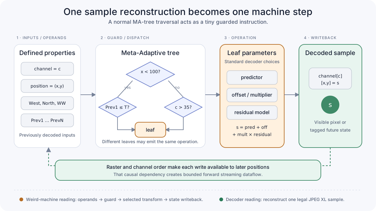
Normal encoders use this machinery to model images efficiently. Our generated tree assigns the same operations CPU roles. Each MA-tree visit is a decode-and-execute step. Coordinate tests select the program phase, threshold tests implement interval lookup tables, and leaf predictors plus offsets act as a small ALU. West, north, west-of-west, and previous-channel references move values through the datapath. Tagged integer ranges distinguish data words from control phases, while the raster itself supplies storage.
The channels provide a strict causal pipeline:
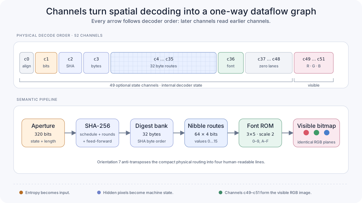
In the final file, hidden channels c0..c48 hold the machinery and visible channels c49..c51 are RGB. c0 consumes three inert one-bit visits needed for bit alignment. c1 receives the 320 meaningful aperture bits. c2 performs the SHA-256 continuation. c3 banks the resulting 32 digest bytes. Channels c4..c35 route one byte apiece and split it into two nibbles. c36 converts nibble tags into visible glyph pixels. Channels c37..c48 are zero-valued budget lanes, and the last three channels copy the bitmap into identical red, green, and blue planes.
Those optional channels form the processor’s state lanes and wires. Every required value travels through defined samples and the format’s dependency graph. The codestream creates the CPU by assigning computational roles to documented decode operations.
So what kind of CPU did we build?
The answer is a finite, unrolled processor specialized for one program. The MA tree is its compiled control logic. The decoder’s monotonic (channel, y, x) traversal supplies a clock and program counter. Earlier samples hold state, while tree leaves implement moves, constants, lookup tables, tagged arithmetic, and writeback.
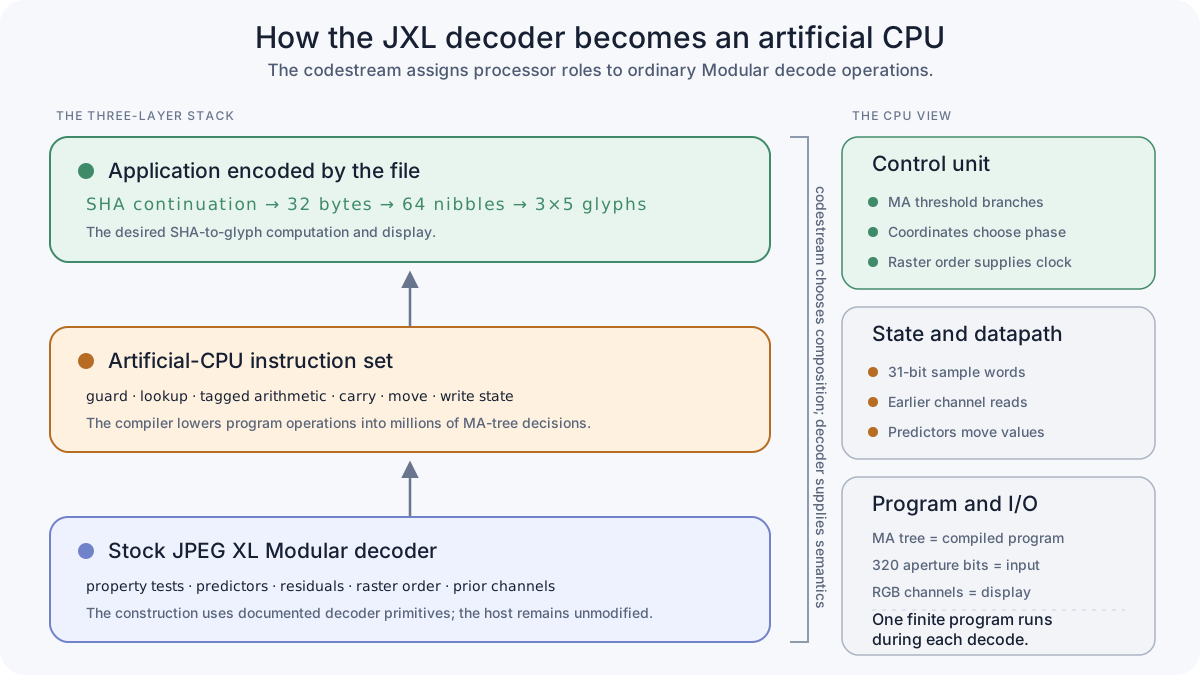
| JPEG XL mechanism | Artificial-CPU role |
|---|---|
| MA-tree threshold test | conditional branch |
| leaf predictor and offset | instruction, ALU operation, or constant |
| west, north, and PrevN samples | registers, wires, and state loads |
| coordinate and channel number | clock, program counter, and pipeline stage |
| tagged 31-bit sample | typed machine word |
| 320 entropy-aperture bits | input tape |
| final RGB samples | output device |
The CPU lasts for one decode. Its address space is the image’s declared sample planes, its input comes from the codestream, and its output device is the RGB image. Image dimensions, channel count, MA-tree size, and the one-way dependency graph fix its capacity. Security literature sometimes calls an unexpected computational interpretation like this a format-semantic weird machine; “artificial CPU” captures the concrete architecture visible here.
Now make the CPU print its own hash
Here comes the self-reference problem. The visible digest depends on the bytes that encode the display, and those bytes contribute to the digest. SHA-256’s iterative chaining structure gives us a clean feed-forward construction. It processes 64-byte blocks while maintaining eight 32-bit chaining words. Let the final file be:
F = P || S
P is the already-fixed prefix, padded at the container level so its length is an exact multiple of 64 bytes. Let H_P be the eight-word SHA-256 state immediately after processing P and before final message padding. The 40-byte suffix placed in the decoder’s entropy aperture is:
S = BE32(H_P[0]) || … || BE32(H_P[7]) || BE64(bit_length(F))
The final artifact is 11,714,152 bytes. Its prefix is 11,714,112 bytes, or 183,033 SHA blocks, and the encoded bit length is 93,713,216. After the 40-byte suffix, standard SHA-256 padding contributes 0x80, fifteen zero bytes, and the same eight-byte length. Therefore the file digest is exactly one known continuation:
SHA256(F) = Compress(
    H_P,
    S || 0x80 || 15 zero bytes || BE64(bit_length(F))
)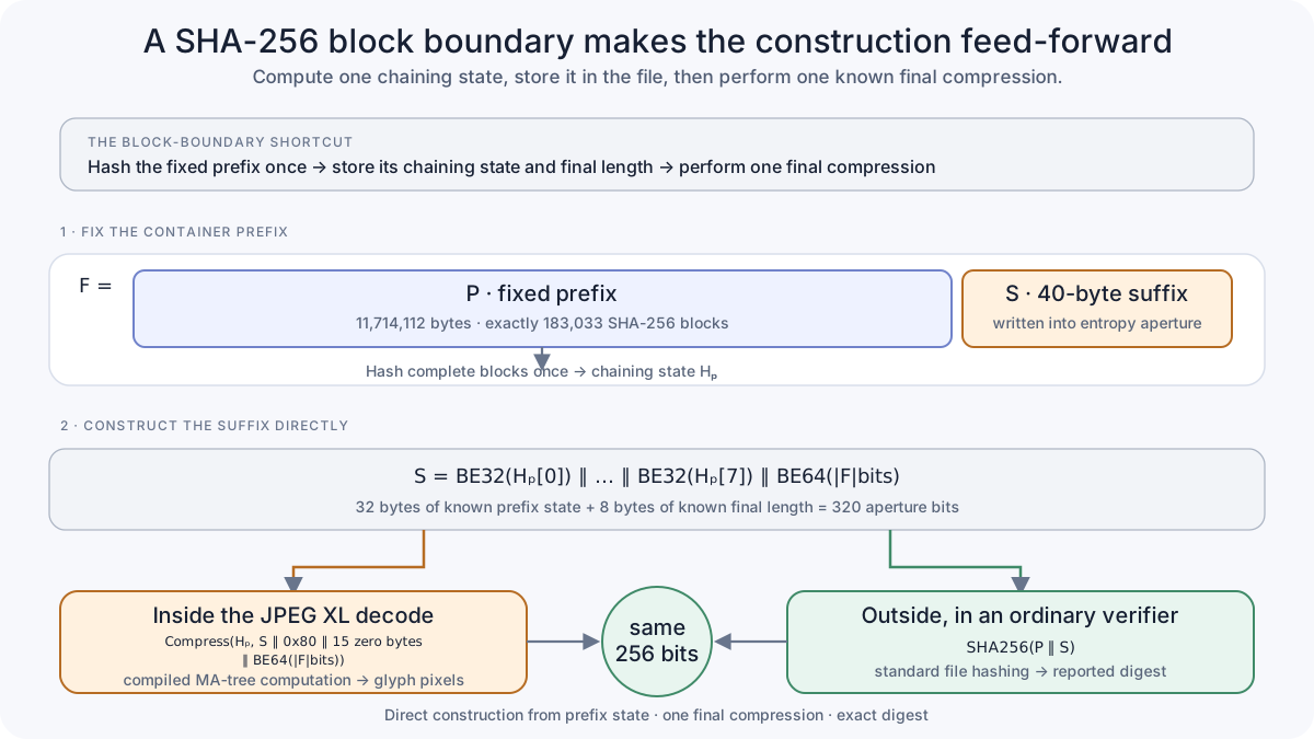
The suffix affects the hash and supplies precisely the state and length needed to compute that hash. Once P and the file length are fixed, S follows directly: hash the prefix, write the suffix, and perform one compression.
The entropy stream contains 323 relevant one-bit visits: three harmless alignment visits followed by a contiguous, byte-aligned 320-bit aperture. A patched authoring encoder installs the 40 bytes above. During decoding, c1 recovers those same bits and hands them to the in-format machine.
Compiling SHA-256 for the JXL CPU
This is where the compiler work gets big. SHA-256 expects 32-bit rotates, Boolean functions, modular addition, a 64-word message schedule, and 64 compression rounds. The compiler lowers each operation into smaller finite mappings built from MA-tree primitives.
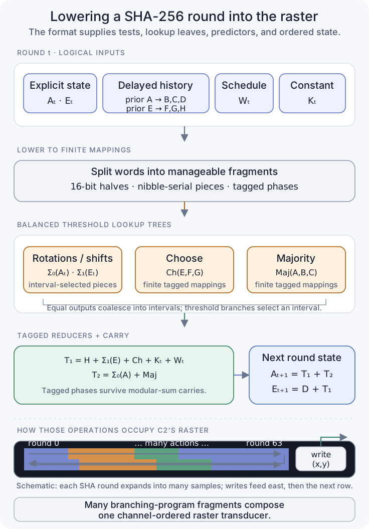
The machine represents a 32-bit word as smaller pieces, including 16-bit halves and nibble-serial fragments. Unary lookup tables map every possible 16-bit source value to a contribution such as a rotated fragment, a Choose term, or a Majority term. Equal consecutive outputs are coalesced into intervals; balanced threshold branches then select the right interval. Small reducers combine tagged contributions while preserving enough phase information to distinguish schedule work, round work, carries, and feed-forward.
State advances west to east and then row to row. The layout stores the evolving A and E sequences explicitly and recovers the other six SHA working words as positionally delayed versions of earlier state. The compiler materializes the final-block message schedule, all 64 rounds, and the feed-forward addition that produces the eight digest words. A coordinate ROM places 9,156 actions, including 2,512 target-state updates and 1,925 tag normalizations, into the raster.
Every reachable tagged value was checked to fit the signed 31-bit sample domain. The generated MA tree has 3,388,159 nodes, 1,694,080 leaves, and maximum depth 34. JPEG XL’s hard ceiling here is 4,194,303 nodes, but libjxl also applies a size-and-channel-dependent ceiling. For this 1024×1024, 52-channel image that effective limit is 3,408,896, leaving 20,737 nodes of margin. The twelve zero lanes raise the channel-dependent node budget and resolve to invisible zero-valued samples.
The output device: hexadecimal pixels
After all that machinery, the display stage is pleasantly simple. SHA-256 emits 32 bytes, each byte splits naturally into two hexadecimal characters, and 64 compact glyphs fit comfortably into the image.
Channel c3 places the bytes in SHA order at a fixed byte bank. Each of c4..c35 owns one byte, extracts its high and low nibbles, and routes two tags in the range 0 through 15. Channel c36 is a direct font ROM for uppercase 0–9 and A–F. Each symbol is a 3×5 bitmap enlarged by a factor of two. The mapping runs directly from bytes to nibbles to glyphs.
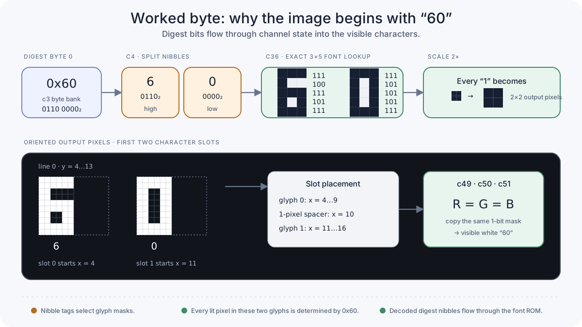
The encoded orientation is 7, which anti-transposes the compact physical routing area into four normal reading lines. In the oriented image, line starts are at y = 4, 16, 28, 40; groups of four characters receive a little extra horizontal spacing. The inclusive lit-pixel bounds are (4,4)..(120,49).
Verifying the program and its output
Then we checked the construction from both ends. The final file’s SHA-256 is:
60f8d1326acd2103903424860c5a64186f947d4fd85dd7c465b7da53c4cbe048
An independent verifier derived the expected glyph pixels from those exact file bytes, decoded the file with unmodified djxl 0.11.2, and OCRed all 64 characters. The observed text matched the digest case-insensitively. It also compared the entire 1024×1024 bitmap: every expected white pixel appeared, every background pixel remained black, all RGB samples were binary, and all three color channels were identical.
The oriented image contains 2,632 lit pixels. Packing its binary mask row-major and most-significant-bit first gives SHA-256:
30ecc016adea8add091a948dcc2c47736411b32c4ea69326c3d38aff76f8a292
The human-readable source tree is 244,199,148 bytes; the serialized naked codestream is about 11.7 MB, and the final JXL container is exactly 11,714,152 bytes.
Specialized compiler, stock decoder
The workflow has two halves: a specialized compiler writes the codestream, and stock decoders run it. The source tree was serialized with a developer build of libjxl at commit 6e0282c3eaeee7abff6c54cfe19e6ac63e9c3316. Its author-side changes expose the large custom tree and raw one-bit aperture, raise the tool’s optional-channel allowance, and make encoding millions of nodes practical. Every operation needed during playback already belongs to the normal decoder.
Acceptance used stock libjxl 0.11.2. The exact artifact also passed the stock ImageIO framework on macOS 26.4, build 25E246, recovering all 64 glyphs and the pinned full mask. The codestream carries the construction, and the decoder supplies the standard Modular semantics.
In a reported iMessage test, the file displayed successfully on stock iOS 26.6. To verify the transfer byte for byte, hash the received attachment and compare its full bitmap with the supplied XCTest. That also reveals whether iMessage kept the original JXL or delivered a rendered derivative.
On macOS, the latest ImageIO run reached 3,338,649,600 bytes maximum resident set size and a 3,379,876,088-byte peak memory footprint — about 3.11 GiB and 3.15 GiB respectively. Comparable iOS memory figures will require an instrumented run.
What the artificial CPU demonstrates
If there is one idea to take away, it is that file formats are small languages and decoders are their interpreters. Prediction, context modeling, optional channels, and ordered reconstruction look like compression details one at a time. Composed carefully, they provide conditionals, lookup tables, state, and dataflow.
JPEG XL supplies this construction with an instruction decoder, 31-bit words, state lanes, a fixed execution schedule, and a pixel display. The codestream wires those components into a purpose-built artificial CPU. Its ROBP-style selectors complete SHA-256, split the digest into hexadecimal nibbles, and draw the result — entirely as ordinary image reconstruction.